Brief book review: Genius at play (Roberts)

9781620405956

Roberts has produced a compelling sketch of Conway both as a highly creative mathematician and as an individual, and somehow also managed to make the fascination of (more or less pure!) mathematics palpable for the layperson. Through their (Roberts and Conway’s) often humorous interactions, we gain a small window into Conway’s background, work ethic, habits, mindset, and struggles (alongside refreshing hints of how at least some of his image was consciously constructed), all of which the academic in me would love to draw some lessons from.

Bonus neuroscience content: Towards the end of the book, they pay a visit to Sandra Witelson, the neuroscientist who has made it her mission to study the brains of individuals thought to have remarkable minds. I am only very loosely acquainted with her work, so I may just be missing the complete picture, but I found myself nodding along to the more skeptical stance of neuroscience-layman Conway in response to some of her thoughts and methods, such as when she said, “I have people asking me whether Einstein’s brain got to be the way it is because he did so much physics. And of course I think it is the other way around. I think he did so much physics because his brain had a certain anatomy.”
I doubt her narrative, but that is far from the point of the book, so I’ll leave it at that. Suffice it to say that I don’t think that her fMRI studies of Conway will produce any meaningful insights into his creative ingenuity.

I took a lot of additional pleasure in the vivid scenes of his life in Cambridge (between the 50s and the 80s), both in the sense of its historical insights, as well as that reminiscent delight of tracing a historical narrative in a physical place that one is (at least slightly) familiar with.

I really enjoyed this trip, and look forward to further encounters with mathematical ideas and concepts (and personalities). (Interestingly, the “beauty and truth” of mathematics, as propagated here, conveniently show the seduction with which certain pockets of theoretical physics may have gotten lost in math.)

Genuis at play: The curious mind of John Horton Conway (Siobhan Roberts)

Further reviews/ratings on Goodreads

Brief book review: Lost in math (Hossenfelder)

97804650942641

This is less of a review and more of a reflection of how the issues raised in this book relate to my area of science. As a psychologist, it is refreshing to learn that psychology’s struggles with theories aren’t unique to psychology (and other social sciences), particularly when precise measurement is a challenge (which it almost always is when your subjects are human beings). As soon as you have difficulty measuring the phenomena that you’re interested in, good old human cognitive biases come into play, regardless of whether you’re a psychologist or physicist, regardless of your mathematical proficiency, regardless of the sophistication of your analytical models.

If particle physicists can be biased by subjective perceptions of mathematical beauty, imagine how much of a struggle it must be to deal with theorists (and outsiders) who feel that they can weigh in on your discussions simply because they have intuitive feelings about the constructs in question, which they may or may not justify with a couple of anecdotes. (Which is not to say that that can never be useful or valid in the process of refining one’s ideas, just that it leads to an inflation of self-assured interjections.)

Of particular interest (but only a brief point in the book) is the observation that this struggle apparently applies not only to theory-building, but also to statistical analyses of empirical observations. Hossenfelder provides examples of multiple published results (in particle physics) that were, in hindsight, probably the result of the type of researcher degrees of freedom that have been identified as a cause for many of the unreliable results (particularly false positive findings) in psychology and co. The fact that it seems to be a relatively new development for collaborations in physics, according to Hossenfelder, “… to settle on a method of analysis before even looking at the data (before the data is ‘unblinded’)” suggests that the current wave of open science measures that seeks to boost reproducibility and replicability in the social sciences isn’t too far behind fields that have typically been perceived as being more methodologically rigorous, and needs to be given time to grow. (Although it is important to stress that most of the core issues of these questionable research practices were known and written about by psychologists decades ago, so none of this is an attempt to absolve the field of its belated response to the blame that it is finally attempting to deal with on a more collective basis.)

There’s a fitting quote often attributed (in different forms) either to Richard Feynman or Murray Gell-Mann: “Imagine how much harder physics would be if electrons had emotions.” I currently don’t have access to any sources to verify whether either (or both, or neither) of them said or wrote that thought, but it sure rings true. As Sanjay Srivastava says, if we were to rethink the common continuum of sciences ranging from “hard” to “soft”, and instead differentiate between “hard” and “easy”, all of the extraneous variables that add complexity to the questions that psychology seeks to answer would probably make it one of the hardest sciences. Alongside theoretical particle physics.

Lost in math: How beauty leads physics astray (Sabine Hossenfelder)

Further reviews/ratings on Goodreads

Brief book review: The songs of trees (Haskell)

61DALStJdEL._SX339_BO1,204,203,200_ “Upend the rain stick and what happens next
Is a music that you never would have known
To listen for. In a cactus stalk …”

Seamus Heaney inadvertently provides an introduction to the premise of Haskell’s book, which expands on the idea of actually paying close acoustic attention to life forms that aren’t usually thought of as producers of sound. He does so by visiting and revisiting a selection of a dozen trees around the world, observing and listening to them and their surroundings through a variety of methods, and using his vast knowledge of nature to put everything into context. And the way that he unpacks this context is the main point of the book.

I was absolutely enchanted by Haskell’s first effort, ‘The Forest Unseen‘. I found the first couple of chapters of ‘The Songs of Trees’ a bit more challenging to get into, but I was more than ready to rhapsodise about it by the end. Haskell once again managed to capture facts of nature in exceedingly beautiful prose. Case in point, this excursion on sea foam: “The foam is made from the pulverized remains of algae and other microscopic life. When these cells break apart in the tumult of the ocean, they release proteins and fats into the water. These chemicals act like soap in a bath, changing the surface tension of water. When the wind agitates the water surface, like a hand whipping a bubble bath, the result is a froth. Sea-foam is a memory of the biology of the ocean, blown to land.”

(Although I did feel that it was a tad bit overdone at certain points — e.g., in describing the information on whether or not to swim in a creek after the rain had added sewage to it, “A click on my social media account tells me whether it would be wise to dunk in this effluvium”).

Regardless, like Haskell and his trees, I definitely plan to revisit both of his books in the future, and I’m already looking forward to it.

“… Who cares if all the music that transpires
Is the fall of grit or dry seeds through a cactus?
You are like a rich man entering heaven
Through the ear of a raindrop. Listen now again.”
(Seamus Heaney, ‘The Rain Stick’)

The songs of trees: Stories from nature’s great connectors (David Haskell)

Further reviews/ratings on Goodreads

Brief book review: Emotional success (DeSteno)

4120C1-UpeL._SX323_BO1,204,203,200_ This book is an easy read, it contains some good ideas and potential information, and it provides some food for thought with regard to its main topic, so I’m not about to advise anyone against checking it out just based on the quibbles that I may have had (some of which may be due to decisions by the publisher/editor to oversimplify some of the content and clearly aim for a pop science flavour to it).

Still, I am afraid that quite a number of points bothered me about this book. I found myself not quite buying some of the interpretations of experimental manipulations. I understand that the descriptions are simplified, so it may very well be that additional manipulation checks just weren’t mentioned, but the issue extended beyond experimental assumptions to interpretations of behaviour in other studies.

If my issues with the book were limited to interpretations, it wouldn’t be quite so bad, but I was also left absolutely unsure about whether the magnitude of the effects were really reported in a fair manner. (For individuals not familiar with statistical methods: the vast majority of psychological differences still result in huge overlap between groups, so simply observing a “difference” doesn’t mean that this difference also has practical relevance.)
I am less concerned about the author’s own studies, but his interpretations of other studies are unfortunately questionable. For example, he introduces the infamous Facebook study, in which emotional content within news feeds was manipulated. The author describes the findings this way: “The results were unambiguous; people’s moods moved towards the contents of their manipulated news feeds. Those who saw more sad posts subsequently posted more sad updates themselves. Those who saw more happy posts showed a similar mirroring.”
Having looked at the actual effects reported in the journal article, these statements are extremely misleading. Yes, the study found “significant” statistical differences. However, these differences were only statistically significant because they had several hundred thousand “participants” to magnify these differences. To draw a direct example from the article: “When positive posts were reduced in the News Feed, … the percentage of words that were negative increased by B = 0.04% (t = 2.71, p = 0.007, d = 0.001)”.
In other words 0.04% = 1 word for every 2,500 words typed across many, many people! That is such a small effect that it is surely hardly worth mentioning, much less presenting as “unambiguous”.

The non-critical description of the Facebook study wasn’t the only point in the book where I found myself questioning either the effect size or the statistical power of the study design of a cited study, which suggests that the author may not have paid attention to these details in at least some of the findings reported in the book (particularly when they weren’t based on studies from his own lab). On top of that, some of the conclusions drawn from fMRI studies seem vastly overstated (with some of them sounding like reverse inferencing).

Casual readers may not place much importance on the next point, but as someone with an interest in the research, I was disappointed in the lack of in-text citations. (I also found it strange that the text cites a particular study by Wilhelm Hofmann several times throughout the book — but at one point introduces Kathleen Vohs, lists her credentials, then describes the study conducted by Hofmann in Germany with words such as “after she studies people’s behavior in their natural environs”, even though it is quite probable that she only played a role in writing the manuscript.)

Overall, I think that the book has many important ideas, but I’m unsure about the strategy of writing in this supposed accessible manner. And for a book meant to summarise other studies, it didn’t do a good job of critically presenting these studies, thus leaving me with too much uncertainty regarding the ideas.

Emotional success: The motivational power of gratitude, compassion and pride (David DeSteno)

Further reviews/ratings on Goodreads

Files and Folders

There are far more detailed guides on file naming and folder organisation out there, but I believe that most people would benefit from two really basic tips.

1.

Consider including the following elements when naming files:

(optional sequence number)_(description)_(date in the format YYYY-MM-DD)_(optional initials of the person who edited this version of the file at the back)

e.g., 02_brief-description_20180125_SK_KS

I consider the date format the most important element of file naming. Files will always be arranged from oldest to latest versions, and you prevent the age-old problem of having files labelled “_final”, “_reallyfinal”, “_toofinaltoofurious”, etc.

2.

Any folder containing files that are being replaced or updated should contain a folder for previous versions of files. This folder would contain all older versions of files that don’t need to be accessed quickly. Ideally, you would be saving a copy of each day’s work to this folder so that nothing gets discarded. The small amount of extra space required for this is absolutely worth it for the relief that you’ll feel (and the regret that you’ll avoid) when the need for a previous version does eventually arise.

e.g.,

aa_old (folder)
00_Manuscript-name_Cover-letter_20180125_KS.docx
01_Manuscript-name_Title-page_20171103_KS.docx
02_Manuscript-name_Main-document_20171212_SK_KS.docx
02_Manuscript-name_Main-document_20180124_KS_SK.docx
02_Manuscript-name_Main-document_20180126_SK_KS.docx
03_Manuscript-name_Supplementary_20171204_KS.docx

aa_old (folder)
00_projectname_raw-data_20171101_KS.sav
01_projectname_data-prep-agg_20171105_KS.sps
01_projectname_data-agg_20171105_KS.sav
02_projectname_data-prep-merg_20171108_KS.sps
03_projectname_data-hypotheses_20171111_KS.sav
04_projectname_Mplus-a_data-prep_20180102_KS.sps
04_projectname_Mplus-b_data-gen_20180102_KS.sps
04_projectname_data_20180102_KS.dat
file-that-has-yet-to-be-sorted.pdf
more-unsorted-files-etc.xlsx
some-sort-of-reference-that-needs-to-be-moved.pdf

Implementing these steps is probably particularly useful when you’re not working alone (particularly when not using options such as Google Docs). Being able to keep track of who added which changes (e.g., easily distinguishing the versions of the file that you completed from the version that your first and second proofreaders just returned to you) and knowing that all previous versions are backed up just a click away has been incredibly helpful to my work process.

Brief book review: How emotions are made (Barrett)

51H-78xDdqL._SX323_BO1,204,203,200_ For outsiders, a lot of neuroscience research can feel like it’s only interesting as foundational/basic research, while the interpretation of social neuroscience, which is presented as being more relevant, can be really frustrating (such as when meaning is assigned to the “activation” of a certain brain area based on what these areas have been linked to in the past — which isn’t appropriate!). The research presented in this book provides a good accessible example of the complementary value of neuroscience research in providing support for a theory that is relevant to our understanding of how we think and feel in our everyday lives.

Having said that, the writing was a tad bit repetitive to me — even beyond the fact that it was written to be accessible for readers with not much knowledge of neuroscience. While mentioning nitpicky points, some of the illustrative examples didn’t quite work for me (although I was able to picture more plausible examples for myself, so these aren’t terrible faults). I’m also unsure about how critically the author looked at studies that she cites to support points that she made outside the context of her own research expertise. For example, she mentions a study on hungry judges several times, although a closer look at the study should prompt skepticism (see this post by Daniel Lakens for the implausibility of the effect size + links to plausible mechanisms/other criticisms). As such, I would be more careful about accepting some of her supporting arguments and recommendations as readily as the ones directly derived from research that she is actually active in. As with the illustrative examples, however, this shouldn’t be seen as a major flaw.

The main point of the book is of course the description of emotions that the author would like to propagate, and the proposed framework definitely provides a lot of food for thought. I must also laud the amount of work that she invested, not just into the extensive references (which should be a given for any serious science writer), but especially into the additional explanations (e.g., of basic neuroanatomy) AND the supporting website that explains some of the points that she makes in even further detail. See https://how-emotions-are-made.com/notes/All_endnotes

How emotions are made: The secret life of the brain (Lisa Feldman Barrett)

Further reviews/ratings on Goodreads

Brief book review: Chaos (Gleick)

519z9hwlHFL A lot has already been said about this classic. I would just like to recommend two videos by the Numberphile channel on YouTube that greatly enhanced my enjoyment of the material covered in the book:

On the Feigenbaum constant https://www.youtube.com/watch?v=ETrYE4MdoLQ

On the chaos game (in the chapter “Images of Chaos”) https://www.youtube.com/watch?v=kbKtFN71Lfs&t

Chaos: Making a new science (James Gleick)

Further reviews/ratings on Goodreads

Statistical Rethinking: Chapter 3

Below are my attempts to work through the solutions for the exercises of Chapter 3 of Richard McElreath’s ‘Statistical Rethinking: A Bayesian course with examples in R and Stan’. If anyone notices any errors (of which there will inevitably be some), I would be happy to be notified!

You can find out more about the book (including a link to full-length lectures!) here.

I won’t post the full details of all questions. Highlighted syntax refers to R code.

The first problems use the samples from the posterior distribution of a globe tossing example (possible values: water or land). This code (from the book + my annotations) provides the specific set of samples.

# This forms the grid for the grid approximation procedure (approximation of the continuous posterior distribution) that we're using in these earlier chapters. This defines a grid of 1000 points.
p_grid <- seq(from=0, to=1 , length.out=1000)   

# This determines the value of the prior at each parameter value on the grid. This case sets a constant prior across all parameter values.
prior <- rep(1, 1000)  

# Likelihood at each parameter value for 6 observations of water from 9 tosses.
likelihood <- dbinom(6, size=9, prob=p_grid) 

# The unstandardised posterior at each parameter value.
posterior <- likelihood * prior 

# The standardised posterior (each value divided by the sum of all values).
posterior <- posterior / sum(posterior)  

# "setting the seed" apparently ensures that the following sample() function produces identical (rather than random) results each time.
set.seed(100)  
samples <- sample(p_grid, prob=posterior, size=1e4, replace=TRUE)

3E1
How much posterior probability lies below p = 0.2?

sum(posterior[p_grid < 0.2])
mean(samples < 0.2)

[1] 0.0008560951
[1] 5e-04

5e-04 = 0.0005
So values below 0.2 (the globe being covered by <20% water) are quite unlikely.

3E2
How much posterior probability lies above p = 0.8?

sum(posterior[p_grid > 0.8])
mean(samples > 0.8)

[1] 0.1203449
[1] 0.1117

3E3
How much posterior probability lies between p = 0.2 and p = 0.8?

sum(posterior[p_grid > 0.2 & p_grid < 0.8])
mean(samples > 0.2 & samples < 0.8)

[1] 0.878799
[1] 0.8878

Corrections to 3E1-3E3 (03.01.19): Jeffrey Girard pointed out that the question specifically says to “use the values in samples” rather than the “posterior” to answer these questions. Thanks, Jeff!

3E4
20% of the posterior probability lies below which value of p?

quantile(samples, 0.2)

20%
0.5195195

3E5
20% of the posterior probability lies above which value of p?

quantile(samples, 0.8)

80%
0.7567568

3E6
Which values of p contain the narrowest interval equal to 66% of the posterior probability?

library(rethinking)

# My understanding of narrowest = the peak of the curve/distribution = highest posterior density interval (HPDI)

HPDI(samples, prob=0.66)

|0.66 0.66|
0.5205205 0.7847848

So about a quarter of the values representing proportion of water (p) provides the central 66% of the probability mass.

3E7
Which values of p contain 66% of the posterior probability, assuming equal posterior probability both below and above the interval?

#  Equal posterior probability requires the regular percentile interval (equal mass on both tails)

PI(samples, prob=0.66)

17% 83%
0.5005005 0.7687688

As the answers in 3E6 and 3E7 are fairly similar, we can conclude that the posterior distribution isn’t too highly skewed in either direction.
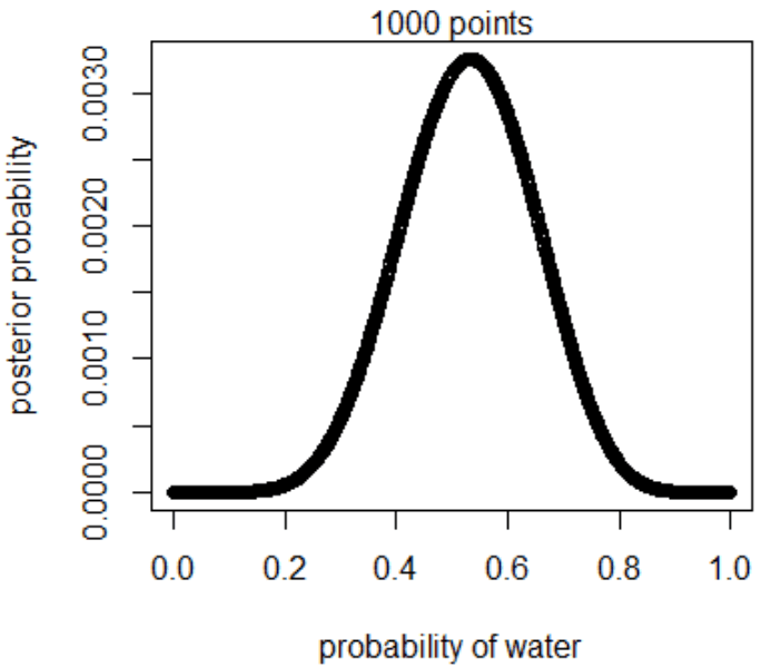
3M1
Suppose the globe tossing data had turned out to be 8 water in 15 tosses. Construct the posterior distribution, using grid approximation. Use the same flat prior as before.

5 steps of grid approximation (these are the same steps that generated the initial sample above):

  1. Define the grid (number of points to estimate the posterior)
  2. Compute prior at each parameter value
  3. Compute likelihood at each parameter value
  4. Compute unstandardised posterior at each parameter value (prior × likelihood)
  5. Standardise the posterior (each value divided by the sum of all values)
p_grid <- seq(from=0, to=1 , length.out=1000) 
prior <- rep(1, 1000)
likelihood <- dbinom(8, size=15, prob=p_grid)   #the only difference to the original code
posterior <- likelihood * prior
posterior <- posterior / sum(posterior)
plot(p_grid, posterior, type="b",
     xlab="probability of water", ylab="posterior probability")
mtext("1000 points")

3M1

3M2
Draw 10,000 samples from the grid approximation from above. Then use the samples to calculate the 90% HPDI for p.

samples <- sample(p_grid, prob=posterior, size=1e4, replace=TRUE)
HPDI(samples, prob=0.9)

|0.9 0.9|
0.3243243 0.7157157

This is the narrowest interval containing 90% of the probability mass

3M3
Construct a posterior predictive check for this model and data. This means simulate the distribution of samples, averaging over the posterior uncertainty in p. What is the probability of observing 8 water in 15 tosses?

# For each sampled value, a random binomial observation is generated. Since the sampled values appear in proportion to their posterior probabilities, the resulting simulated observations are averaged over the posterior. 

ppc <- rbinom(1e4, size=15, prob=samples)

# The probability of observing 8 water in 15 tosses can be summarised as the point estimate. The highest posterior probability, a maximum a posteriori (MAP) estimate.

table(ppc)/1e4

ppc
0 1 2 3 4 5 6 7 8 9 10 11 12
0.0005 0.0037 0.0106 0.0285 0.0539 0.0834 0.1139 0.1412 0.1446 0.1387 0.1095 0.0821 0.0521
13 14 15
0.0281 0.0076 0.0016

The probability of observing 8 water in 15 tosses is 0.1446, which appears to be the biggest probability of all possible values in this sample.

3M4
Using the posterior distribution constructed from the new (8/15) data, now calculate the probability of observing 6 water in 9 tosses.

ppc2 <- rbinom(1e4, size=9, prob=samples)
table(ppc2)/1e4

ppc2
0 1 2 3 4 5 6 7 8 9
0.0047 0.0283 0.0765 0.1441 0.1856 0.2024 0.1769 0.1143 0.0540 0.0132

Observing 6 water in 9 tosses has a probability of 0.1769, which isn’t the most likely value based on this data set.

3M5
Start over at 3M1, but now use a prior that is zero below p = 0.5 and a constant above p = 0.5. This corresponds to prior information that a majority of the Earth’s surface is water. Repeat each problem above and compare the inferences. What difference does the better prior make? If it helps, compare inferences (using both priors) to the true value p = 0.7.


p_grid <- seq(from=0, to=1 , length.out=1000) 
prior <- ifelse(p_grid < 0.5, 0, 1)      # zero below p = 0.5 and constant above
likelihood <- dbinom(8, size=15, prob=p_grid)   
posterior <- likelihood * prior
posterior <- posterior / sum(posterior)

samples <- sample(p_grid, prob=posterior, size=1e4, replace=TRUE)
HPDI(samples, prob=0.9)

|0.9 0.9|
0.5005005 0.7137137

The range has been narrowed down.

ppc <- rbinom(1e4, size=15, prob=samples)
table(ppc)/1e4

ppc
1 2 3 4 5 6 7 8 9 10 11 12 13
0.0001 0.0007 0.0035 0.0116 0.0355 0.0615 0.1138 0.1571 0.1779 0.1675 0.1291 0.0854 0.0380
14 15
0.0150 0.0033

8 is slightly more likely than before, yet no longer the most likely number. The prior affects the interpretation of the data. Although 70% of 15 is 10.5, so the new prior isn’t quiiite there yet.

ppc2 <- rbinom(1e4, size=9, prob=samples)
table(ppc2)/1e4

ppc2
0 1 2 3 4 5 6 7 8 9
0.0007 0.0050 0.0258 0.0780 0.1582 0.2268 0.2403 0.1650 0.0829 0.0173

6 is now the most probable observation in 9 tosses. (70% of 9 is 6.3, so that’s fairly close.)
For fun, let’s try a slightly more exact prior:

p_grid <- seq(from=0, to=1 , length.out=1000) 
prior <- ifelse(p_grid < 0.6, 0, 0.7)
likelihood <- dbinom(8, size=15, prob=p_grid)  
posterior <- likelihood * prior
posterior <- posterior / sum(posterior)
 
samples <- sample(p_grid, prob=posterior, size=1e4, replace=TRUE)
HPDI(samples, prob=0.9)

|0.9 0.9|
0.6006006 0.7467467

ppc <- rbinom(1e4, size=15, prob=samples)
table(ppc)/1e4

ppc
2 3 4 5 6 7 8 9 10 11 12 13 14
0.0001 0.0006 0.0031 0.0092 0.0268 0.0629 0.1139 0.1659 0.2006 0.1858 0.1265 0.0701 0.0285
15
0.0060

Bingo!

ppc2 <- rbinom(1e4, size=9, prob=samples)
table(ppc2)/1e4

ppc2
0 1 2 3 4 5 6 7 8 9
0.0002 0.0018 0.0092 0.0389 0.1031 0.2022 0.2463 0.2407 0.1236 0.0340

That’s more like it!

Okay, the next problems require a different data set, which basically specifies the sex of child 1 and child 2 from 100 two-child families.

library(rethinking)
data(homeworkch3)

3H1
Using grid approximation, compute the posterior distribution for the probability of a birth being a boy. Assume a uniform prior probability. Which parameter value maximizes the posterior probability?

birthboys <- sum(birth1, birth2)
p_grid <- seq(from=0, to=1, length.out=1000) 
prior <- rep( 1, 200) 
likelihood <- dbinom(birthboys, size=200, prob=p_grid) 
unstd.posterior <- likelihood * prior 
posterior <- unstd.posterior / sum(unstd.posterior) 

plot(p_grid, posterior, type="b",
     xlab="probability of boy birth", ylab="posterior probability")

3H1

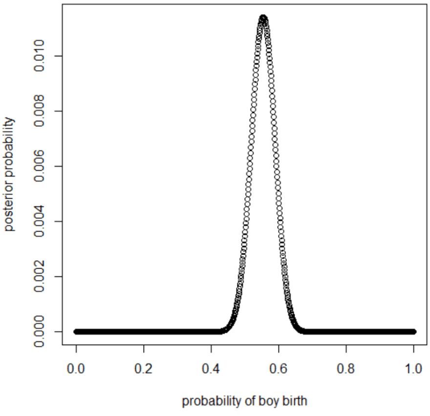
p_grid[which.max(posterior)]

[1] 0.5545546

3H2
Using the sample function, draw 10,000 random parameter values from the posterior distribution you calculated above. Use these samples to estimate the 50%, 89%, and 97% highest posterior density intervals.

samples <- sample(p_grid, size=1e4, replace=TRUE, prob=posterior)

# HPDI = narrowest interval containing the specified probability mass.

HPDI(samples, prob=0.50)

|0.5 0.5|
0.5313531 0.5771577

HPDI(samples, prob=0.89)

|0.89 0.89|
0.4981498 0.6079608

HPDI(samples, prob=0.97)

|0.97 0.97|
0.4830483 0.6315632

3H3
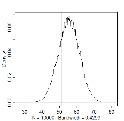
Use rbinom to simulate 10,000 replicates of 200 births. You should end up with 10,000 numbers, each one a count of boys out of 200 births. Compare the distribution of predicted numbers of boys to the actual count in the data (111 boys out of 200 births). There are many good ways to visualize the simulations, but the dens command (part of the rethinking package) is probably the easiest way in this case. Does it look like the model fits the data well? That is, does the distribution of predictions include the actual observation as a central, likely outcome?

simulation <- rbinom(1e4, size=200, prob=samples)
dens(simulation)
abline(v=111)

3H3

The distribution of predictions does seem to include the actual observation as a central outcome.

3H4
Now compare 10,000 counts of boys from 100 simulated first borns only to the number of boys in the first births, birth1. How does the model look in this light?

birth1sum <- sum(birth1)
likelihood2 <- dbinom(birth1sum, size=100, prob=p_grid) 
prior2 <- rep( 1, 100) 
unstd.posterior2 <- likelihood2 * prior2 
posterior2 <- unstd.posterior2 / sum(unstd.posterior2) 
samples2 <- sample(p_grid, size=1e4, replace=TRUE, prob=posterior2)

simulation2 <- rbinom(1e4, size=100, prob=samples2)
dens(simulation2)
abline(v=51)

3H4a

If this was the intended interpretation, the distribution of predictions seems to include the actual observation as a central outcome here, too.
However, the question could also be interpreted differently. Here is a simulation based on the randomly pulled samples from the vector of the posterior density of the initial estimate of the whole sample:

simulation3 <- rbinom(1e4, size=100, prob=samples)
dens(simulation3)
abline(v=51)

3H4b

The actual number of boys appears to be below this estimation, indicating that the posterior density based on the whole sample doesn’t generalise to just first-borns. The next question mentions independence of first and second births as an assumption, although this finding already seems to contradict it.

3H5
The model assumes that sex of first and second births are independent. To check this assumption, focus now on second births that followed female first borns. Compare 10,000 simulated counts of boys to only those second births that followed girls.

firstgirls <- 100 - sum(birth1)     # number of female first-borns: 49
boysaftgirls <- birth2[birth1==0]   # this gathers the corresponding second-borns who followed a female first-born
simulation4 <- rbinom(1e4, size=firstgirls, prob=samples)
dens(simulation4)
abline(v=sum(boysaftgirls))  # the "sum" function here gives meaning to the "boys after girls" name

3H5

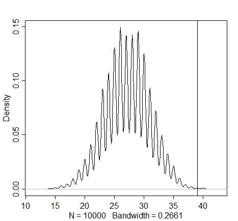
Here we see further evidence for the contradiction of the assumption of independence (as observed in the previous graph). The actual number of male births that follow the female births seems much higher than one would expect when assuming that first and second births are independent. As the first births seem to be divided relatively equally, these parents appear to have dabbled in sex selection.

Statistical Rethinking: Chapter 2

Below are my attempts to work through the solutions for the exercises of Chapter 2 of Richard McElreath’s ‘Statistical Rethinking: A Bayesian course with examples in R and Stan’. If anyone notices any errors (of which there will inevitably be some), I would be happy to be notified!

You can find out more about the book (including links to full-length lectures) here.

Note: I completed Chapter 2 several weeks ago, and I can’t find my answers to the “medium” level questions (I think I calculated some of them by hand), so I’ll start at the “hard” ones this time.

I’m not going to post the full questions. Highlighted syntax refers to R code.

2H1
Species A gives birth to twins 10% of the time, otherwise birthing a single infant.
Species B births twins 20% of the time, otherwise birthing singleton infants.
A female panda of unknown species has just given birth to twins. What is the probability that her next birth will also be twins?

pr_A_T <- 0.1  # probability of species A producing twins
pr_B_T <- 0.2  # probability of species B producing twins
prior_AorB <- 0.5  # prior probability of it being either species A or B
# probability of two twin births in a row = posterior probability of twins for species A + posterior probability of twins for species B
# posterior probability of twins for species A = (probability of species A producing twins * prior) / probability of twins at a single point of time

# probability of twins at a single point of time (without prior knowledge)
pr_twins <- (pr_A_T * prior_AorB + pr_B_T * prior_AorB)

pr_T_A <- (pr_A_T * prior_AorB)/(pr_twins)
pr_T_B <- (pr_B_T * prior_AorB)/(pr_twins)
pr_T_T <- (pr_T_A * pr_A_T) + (pr_T_B * pr_B_T)

# Solution: Probability of two twin births in a row

pr_T_T

[1] 0.1666667

This answer seems plausible, considering that it lies between 0.1 and 0.2 (the respective probabilities of species A and B producing twins).

2H2
What is the probability that the panda we have is from species A, assuming we have observed only the first birth and that it was twins?

# We already computed this with the "probability of twins, given species A" function above.
pr_T_A

[1] 0.3333333

It appears less likely (lower than 0.5) for Ms. Panda to be of species A, as species B has a slightly higher tendency of popping out twins. Note that this does not rule out species A — a 1/3 probability should not be underestimated.

2H3
The same panda mother has a second birth and it is not twins, but a singleton infant. What is the posterior probability that this panda is species A?

# probability of first giving birth to twins, then to a singleton in general
pr_NT_T <- 0.1 * 0.9 * 0.5 + 0.2 * 0.8 * 0.5

# probability of twins and then a single baby for species A
pr_TN_A <- 0.1 * 0.9

pr_A_TN <- (pr_TN_A * prior_AorB) / pr_NT_T
pr_A_TN

[1] 0.36

We now have a slight increase in the probability that we’re dealing with species A, thanks to Baby Singleton.

2H4
We now have a genetic test!
The probability that it correctly identifies a species A panda is 0.8.
The probability that it correctly identifies a species B panda is 0.65.
Our panda tests positive for species A.
Part 1: Disregarding the previous information of the births, what is the posterior probability that our panda is species A?
Part 2: Redo calculation using the birth data.

pr_A_A <- 0.8
pr_A_B <- 0.35
pr_B_B <- 0.65
pr_B_A <- 0.2

pr_testA_A <- 0.8
pr_testA <- pr_A_A * prior_AorB + pr_A_B * prior_AorB

pr_A_testA <- (pr_testA_A * prior_AorB) / pr_testA
pr_A_testA

[1] 0.6956522


Edit (28.07.2018): It was brought to my attention that the logic of the solution above isn’t quite clear, so here’s an attempt to put the code into words:

Bayes’s Theorem:
P(really species A|test says A) = P(test says A|really species A)*P(prior) / P(test says A)

or in further detail:

The probability of a true positive identification of species A when the test says “A”
=
(probability of the test saying A when it really is species A [0.8] * probability of it being species A [our prior of 0.5])
divided by
(probability of the test saying A under any circumstances, regardless of whether it’s a true positive or false negative result)

For Part 2, I will simply replace the prior with what we learned in 2H3.

pr_A_A <- 0.8
pr_A_B <- 0.35
pr_B_B <- 0.65
pr_B_A <- 0.2

pr_testA_A <- 0.8
pr_testA <- pr_A_A * pr_A_TN + pr_A_B * (1 - pr_A_TN)

pr_A_testA <- (pr_testA_A * pr_A_TN) / pr_testA

pr_A_testA_TN <- (pr_testA_A * pr_A_TN) / pr_testA
pr_A_testA_TN

[1] 0.5625

When considering our prior knowledge of the actual births, the confidence of the test is now reduced from almost 70% to about 56% that our panda descends from species A (although this is still higher than the probability of 33-36% without the genetic test).

Brief book review: The essential guide to effect sizes (Ellis)

51ve3-1lhoL._SX350_BO1,204,203,200_ Paul Ellis provides a very accessible introduction to several basic topics that are vital to good research practice. In order to encourage readers who enjoyed this book to dive deeper into the literature, I feel the need to point out that the content is slightly out of date on several counts; two points that immediately come to mind are (1) the non-critical presentation (or even the outright recommendation?) of the flawed “fail-safe N” method (see Becker, 2005; Ioannidis, 2008; Sutton, 2009; Ferguson & Heene, 2012 for criticisms, or this Cochrane handbook link for a brief summary) and (2) the lack of mention of viable methods to provide support for null-hypotheses (e.g., equivalence testing or Bayesian methods).

That should, however, not take away from the fact that the text offers an easily comprehensible treatment of the subject matter, and I would recommend it to anyone who happens to be searching for a non-technical introduction to the topics that it covers.

Becker, B. J. (2005). Failsafe N or file-drawer number. In H. R. Rothstein, A. J. Sutton, & M. Borenstein (Eds.), Publication bias in meta-analysis. Sussex: Wiley.
Ferguson, C. J., and Heene, M. (2012). A vast graveyard of undead theories: Publication bias and psychological science’s aversion to the null. Perspectives on Psychological Science, 7, 555–561. doi: 10.1177/1745691612459059
Ioannidis, J. P. A. (2008). Interpretation of tests of heterogeneity and bias in meta-analysis. Journal of Evaluation in Clinical Practice, 14, 951–957. doi: 10.1111/j.1365-2753.2008.00986.x
Sutton, A. J. (2009). Publication bias. In H. Cooper, L. Hedges, and J. Valentine (Eds.), The handbook of research synthesis and meta-analysis (pp. 435–452). New York: Russell Sage Foundation.

The essential guide to effect sizes (Paul Ellis)

Further reviews/ratings on Goodreads